
Matlab
Command Line Terminal
help
format
format dataType指定数字的格式
who
显示当前有哪些变量
whos
显示当前变量的详细信息
clear
清除所有变量,后加变量名则清除单个变量
;
句末加分号,不显示计算结果
方向键
显示历史命令
clc
清屏
time
tic
command
toc
% count the time of runing command
Matrix
矩阵的输入
Row vector:
	a = [1 2 3]
Column vector:
	b = [1;2;3]
Array Indexing
- A(row.column)
- A([row1 row2],[column1 column2]) 得到交集
- A(index)
- A([index1 index2 index3])
- A([index1 index2;index3 index4])
Replacing Entries
delete row: A(row,:) = []
Colon Operator
A = begin:end  => A=[begin begin+1 .... end]
A = begin:i:end => A=[begin begin+i begin+2i ...]
Colon opertator 用作index时代表全部
Array Concatenation
F = [A B]
F = [A;B]
Array Manipulation
with Matirx
- ‘+’ : 同位置相加
- ‘-’ : 同位置相减
- ‘*’ : 前一个矩阵的行与后一个矩阵的列相乘
- ‘/’ : 相当于与逆矩阵做乘法
- .*: 同位置相乘
- ./: 同位置相除
- A’: A的转置
with number
- ‘+’ : 每个entry都加number
- ‘-’ : 每个entry都减number
- ‘*’ : 每个entry都乘number
- ‘/’ : 每个entry都除number
- .*: 同 *
- ./: 同 /
- ^ : n个矩阵相乘
- .^: 每个entry都求n次幂
Special Matrix
- eye(n): n*n identity matrix
- zeros(n1,n2): n1*n2 zero matrix
- ones(n1,n2): n1*n2 matirx with every entry as 1
- diag(): diagonal matrix
- linspace(): linearly spaced vectors
- rand(): uniformly distributed random numbers
Matrix Related Functions
- max(A): find max entry in every column
- max(max(A)):find max entry
- min(A):find min entry in every column
- sum(A):get sum in every column
- mean(A):get average in every column
- sort(A):sort every column of A
- sortrows(A):sort A by first column and exchange rows
- size(A): return row and column
- length(A): vector’s length
- find(A == num): return num’s index
Structured programming
if elseif else
if condition1
	statement1
elseif condition2
	statement2
else
	statement3
end
switch
switch expression
case value1
	statement1
case value2
	statement2
otherwise
	statement3
end
while
while condition
	statement
end
for
for variable = start : increment : end
	commands
end
break
terminates the execution of for or while loops
Tips
- At the beginning of the script, use command
- clear all to remove previous varibles
- close all to close all figures
- clc to clear history
- Use semicolon ; at the end of commands to inhibit unwanted output
- Use ellipsis … to make scripts more readable
- Ctrl+C to terminate the running script
Function
example
% function name = file name
function y = freebody(x0, v0, t)
x = x0 + v0.*t + 1/2*9.8*t.*t;
function [a F] = acc(v2, v1, t2, t1, m)
a = (v2 - v1)./(t2 - t1);
F = m.*a;

[Acc Force] = acc(20, 10, 5, 4, 1)
Function default variables
-
inputname
Variable name of function input
-
mfilename
File name of currently running function
-
nargin
Number of function input arguments
-
nargout
Number of function out arguments
-
varargin
Variable length input argument list
-
varargout
Variable length out argument list
Function handles
A handle is a pointer to a function
A way to create anonymous function
f = @(x) exp(-2*x);
x = 0:0.1:2;
% draw figure
plot(x, f(x))
Variables
-
numeric
- int8, int16, int32, int64
- uint8, uint16, uint32, uint64
- single
- double
-
char
% char is represented in ASCII using a numeric code between 0 to 255 a = 'c' % declare string variable str = 'abcdeabc' str(3) % print 'c' , 3 as index str == 'a' % print 1 0 0 0 1 0 0 str(str == 'a') = 'Z' % a -> Z print 'ZbcdZbc' -
logical
-
cell
-
structure
-
function handle
Structure
declare
% 1
student.id = 'first';
student.name = 'first';
student.number = 123456;
student.grade = [100, 75, 73;...
				95, 91, 85.5;...
				100, 98, 72];
student

student(2).id = 'second';
student(2).name = 'second';
student(2).number = 123456;
student(2).grade = [100, 75, 73;...
                   95, 91, 85.5;...
                   100, 98, 72];

% 2
A = struct('data', [3 4 5;8 0 1],...
			'nest', struct('x', [1 2 3], ...
						   'y', [3 4 5]));
% A.data = [3 4 5;8 0 1]
% A.nest.x = [1 2 3]
% A.nest.y = [3 4 5]
Structure Function
- fieldnames(S) : get all the fildnames of S
- rmfield(S, ‘id’) : remove the field ‘id’ of S
Cell
delare
delared using {}
% 1
A(1,1) = {[1 2;3 4]};
A(1,2) = {'string'};
A(2,1) = {3+7i};
A(2,2) = {-pi:pi:pi};
A

% 2
A{1,1} = [1 2;3 4];
A{1,2} = 'string';
A{2,1} = 3+7i;
A{2,2} = -pi:pi:pi;
A
Accessing cell array
A(1,1)
% return a cell data

A{1,1}
% return the content in the cell
Cell Array Function
- cell(row,column) : create cell array
- cell2struct : convert cell array to structure
- mat2cell : convert array to cell array with different sized cells
- num2cell : convert array to cell array with consistently sized cells
- cat(dimension,A,B) : concat cell array in different dimensions
- reshape(A,row,column) : reshape cell array
Type Convertion
- double()
- single()
- int8() int16() int32() int64()
- uint8() uint16() uint32() uint64()
File Access
| File Content | Extension | Description | Import Function | Export Function |
|---|---|---|---|---|
| mat | saved matlab work space | load | save | |
| Text | space delimited numbers | load | save | |
| SpreadSheet | xls, xlsx | xlsread | xlswrite |
save
-
work space
save filename.mat % save workspace data in file save filename.mat -ascii % save readable workspace data in file -
xls
xlswrite('filename.xlsx', variable, sheet_page, location)

% example
xlswrite('filename.xlsx', M, 1, 'E2:E4') % M is a matrix
xlswrite('filename.xlsx', {'Mean'}, 1, 'E1')
load
-
work space
load ('filename.mat') load ('filename.mat', '-ascii') -
xls
score = xlsread('filename.xlsx')

score = xlsread('filename.xlsx', 'B2:D4')

[score header] = xlsread('filename.xlsx')
Low-level File I/O Functions
- fopen
- fclose
- fscanf
- fprintf
- feof
% example
x = 0:pi/10:pi;y = sin(x);
fid = fopen('filename.txt', 'w');
for i=1:11
	fprintf(fid, '%5.3f %8.4f\n', x(i), y(i));
end
fclose(fid);
plot
plot()
- plot(x, y) : plot each vector pairs (x,y)
- plot(y) : plot each vector pairs (x,y) where x = [1 … n] ,n=length(y)
hold on/off
use hold on to have both plots in one figure
hold on
plot(cos(0:pi/20:2*pi))
plot(sin(0:pi/20:2*pi))
hold off
plot style
plot(x, y, 'str')
LineSpec (MATLAB Functions) (northwestern.edu)
- Data markers
- dot : .
- cross : X
- circle : O
- plus sign : +
- Line types
- solid line : -
- dashed line : –
- dash-dotted line : -.
- dotted line : :
- Colors
- black : k
- $\color{#0000FF}{蓝}$ : b
- cyan : c
- green : g
- magenta : m
- red : r
- white : w
- yellow : y
legend()
add legend to graph
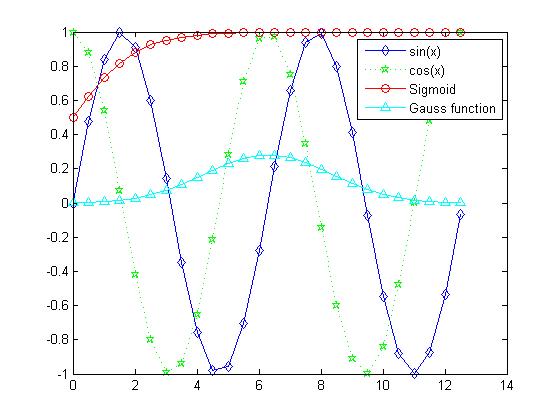
plot(x,y,'bd-', x,h,'gp:')
legend('L1', 'L2')
title & label
- title()
- xlabel()
- ylabel()
- zlabel()
text & annotation
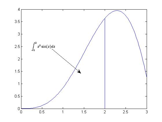
str = '$$ \int_{0}^{2} x^2\sin(x) dx $$';
text(x, y, str, 'Interpreter', 'latex');
annotation('arrow', 'X', [0.32,0.5], 'Y', [0.6,0.4]);
figure adjustment
Identifying the handle of an object
- h = plot(x,y);
- Utility functions
- gca : return the handle of the current axes
- gcf : return the handle of the current figure
- allchild : Find all children of specified objects
- ancestor : Find ancestor of graphics object
- delete : delete an object
- findall : find all graphics objects
Fetching or Mordifying properties
-
fetch properties : get()
h = plot(x,y); % get line properties get(h); % get axes properties get(gca) % get figure properties get(gcf) -
modify properties : set()
set(handle, property, value)
properties
- Axes
- FontSize
- XTick
- XTickLabel
- FontName
- Line
- LineStyle
- LineWidth
- Color
- Figure
- Position : [left, bottom, width, height]
Mutiple plots
-
serval plots in different figures
figure, plot(x, y1); figure, plot(x, y2); -
serval plots in **a figure **
% subplot(row, column, num)
subplot(2,2,1); plot(x,y); axis normal
subplot(2,2,2); plot(x,y); axis square
subplot(2,2,3); plot(x,y); axis equal
subplot(2,2,4); plot(x,y); axis equal tight
Control of Grid, Box and Axis
- grid on/off
- box on/off
- axis on/off
- axis normal
- axis square
- axis equal
- axis equal tight
Save figures
-
saveas(gcf, 'filename', 'formattype') -
print
Option
- Bitmap
- jpeg
- png
- tiff
- bmpmono
- bmp
- Vector
- eps
- epsc
- meta
- svg
- ps
- psc
Advanced 2D plots
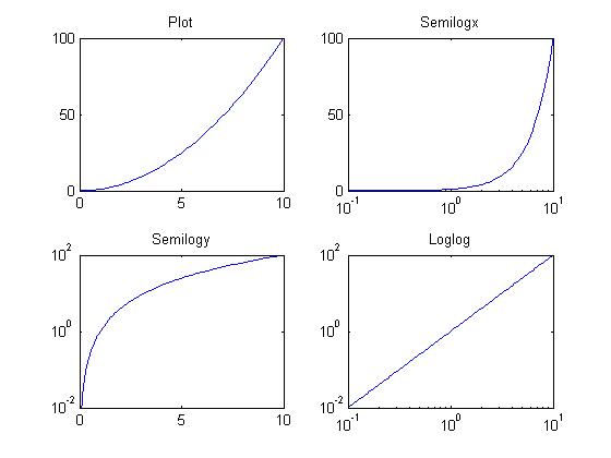
Logarithm Plots
Take the logarithm of the axis
- semilogx
- semilogy
- loglog
plotyy
two y axis
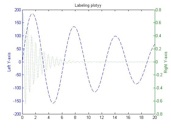
[AX, H1, H2] = plotyy(x,y1,x,y2);
set(get(AX(1), 'Ylabel'), 'String','Left Y-axis');
set(get(AX(2), 'Ylabel'), 'String','Right Y-axis');
set(H1, 'LineStyle', '--'); set(H2, 'LineStyle', ':');
graph
-
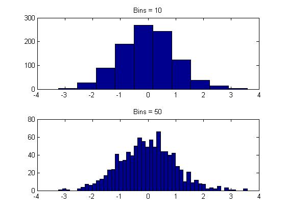
Histogram
- hist(y, bins)
-
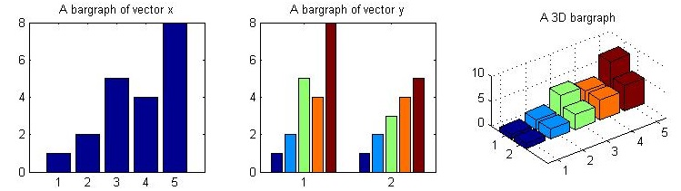
bar chart
- bar(y) : create a bar chart of y
- bar3(y) : create a 3D bar chart of y
- bar(y, ‘stacked’) : create a stacked bar chart of y
- barh(y) : create a hrizontal bar chart of y
-
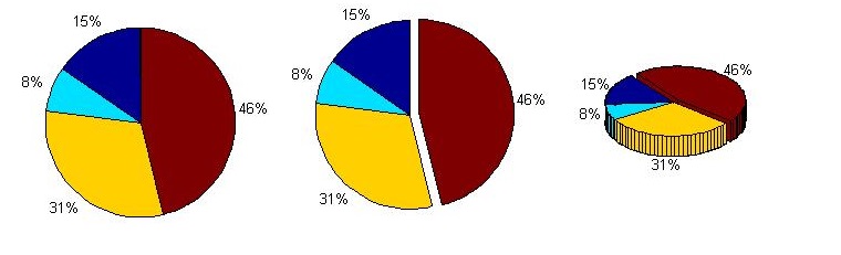
pie chart
- pie(a) : create a pie chart
- pie(a,[0,0,0,1]) : create a pie chart and ‘1’ is a separated section
- pie3(a) : create a 3d pie chart
-
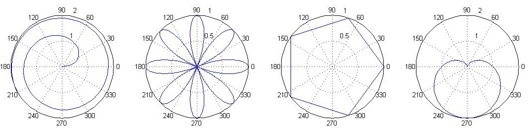
polar chart
- polar(theta, r)
-
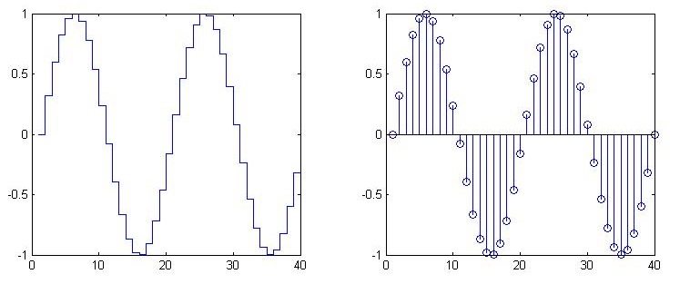
stairs and stem chart
- staris(y)
- stem(y)
-
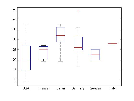
boxplot
- boxplot(MPG, Origin)
-
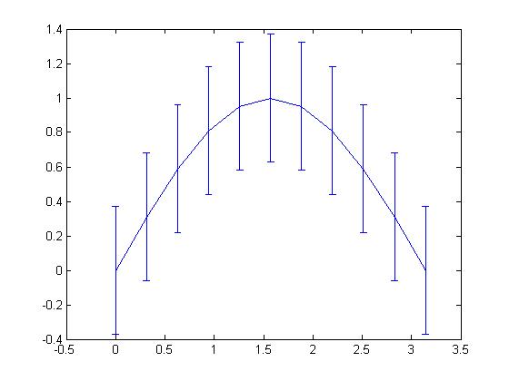
error bar
- errorbar(x,y,e)
color
fill
t = (1:2:15)*pi/8; x = sin(t); y = cos(t)
fill(x,y,'r'); axis square off;
text(0,0,'STOP','Color','w','FontSize',80 ...
	'FontWeight','bold','HorizontalAlignment','center');
color space
[R G B]
color bar
colorbar;
Display the color of the gradation
imagesc
Convert the element values in matrix A to different colors by size : imagesc(A)
clormap
set the current colormap colormap([name])

3D plots
plot3
plot3(x,y1,z1,'r',x,y2,z2,'b');
meshgrid
create two matrices that satisfy the following conditions
- the same for each row of x
- the same for each column of y
- The length of vector x is the number of **columns** of the new matrix
- The length of vector y is the number of **rows** of the new matrix
[X,Y] = meshgrid(x,y);
% x = [1 2 3]; y = [4 5]
% X = [1 2 3;1 2 3] y = [4 4 4;5 5 5]
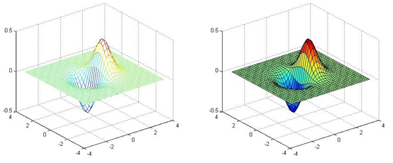
Surface Plots
- mesh()
- surf()
- meshc() : add contour at the bottom
- surfc()
x = -3.5:0.2:3.5; y = -3.5:0.2:3.5;
[X,Y] = meshgrid(x,y);
Z = X.*exp(-X.^2-Y.^2);
subplot(1,2,1); mesh(X,Y,Z);
subplot(1,2,2); surf(X,Y,Z);
contour
Draw contour lines of 3D graphics
- contour()
- Clabel() : Add elevation labels to contour plots
- contourf() : fill color
view
vary the view angle
view(Azimuth, Elevation)
light
% example

% provide a light
L1 = light('Position',[-1 -1 -1]);

% set the light that have been provided
set(L1, 'Position', [-1 -1 1]);

%set the color of light
set(L1, 'Color', 'g');
Digital Image
Type
- Binary Image : 0 is balck and 1 is white
- Greyscale Image : one channel , 0 to 255, black to white
- Color Image : three channel , R G B
Read and Show Image
-
Read an image : imread()
-
Show an image : imshow()
I = imread('file'); % I is an image matrix
imshow(I);
Image info
imageinfo(file)
Write Image
imwrite(I, 'filename.png')
Image Processing
Image Arithmetic
- imadd
- imsubtract
- immultiply
- imdivide
- imcoplement
Image Histogram
-
imhist
imhist(I)Display the grayscale histogram of image i -
histeq
I1 = histeq(I)histeq can produce an image with an average gray level distribution probability
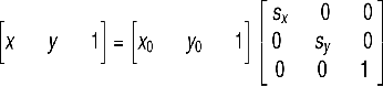
Geometric Transformation
| Transform | Example | Transfomation Matirx | command |
|---|---|---|---|
| Translation |  |
 |
imtranslate() |
| Scale |  |
 |
imresize() |
| Shear |  |
- | |
| Rotation |  |
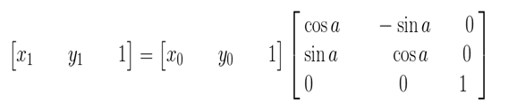 |
imrotate() |
Image thresholding
if pixel < threshold ,
pixel = black,
else pixel = white
-
graythresh() : computes an optimal threshold
-
im2bw() : converts an images into binary images
I = imread('file.png');
level = graythresh(I);
bw = im2bw(I,level);
Background Estimation
Estimation for the gray level of the background
BG = imopen(I,strel('disk',15));
imshow(BG);
Background subtraction
If thresholding the inital image, some item will be subtracted and some background will be remained as dot
So, subtract background to optimize the image thresholding
I2 = imsubtract(I,BG);
Connected-component labeling : bwlabel()
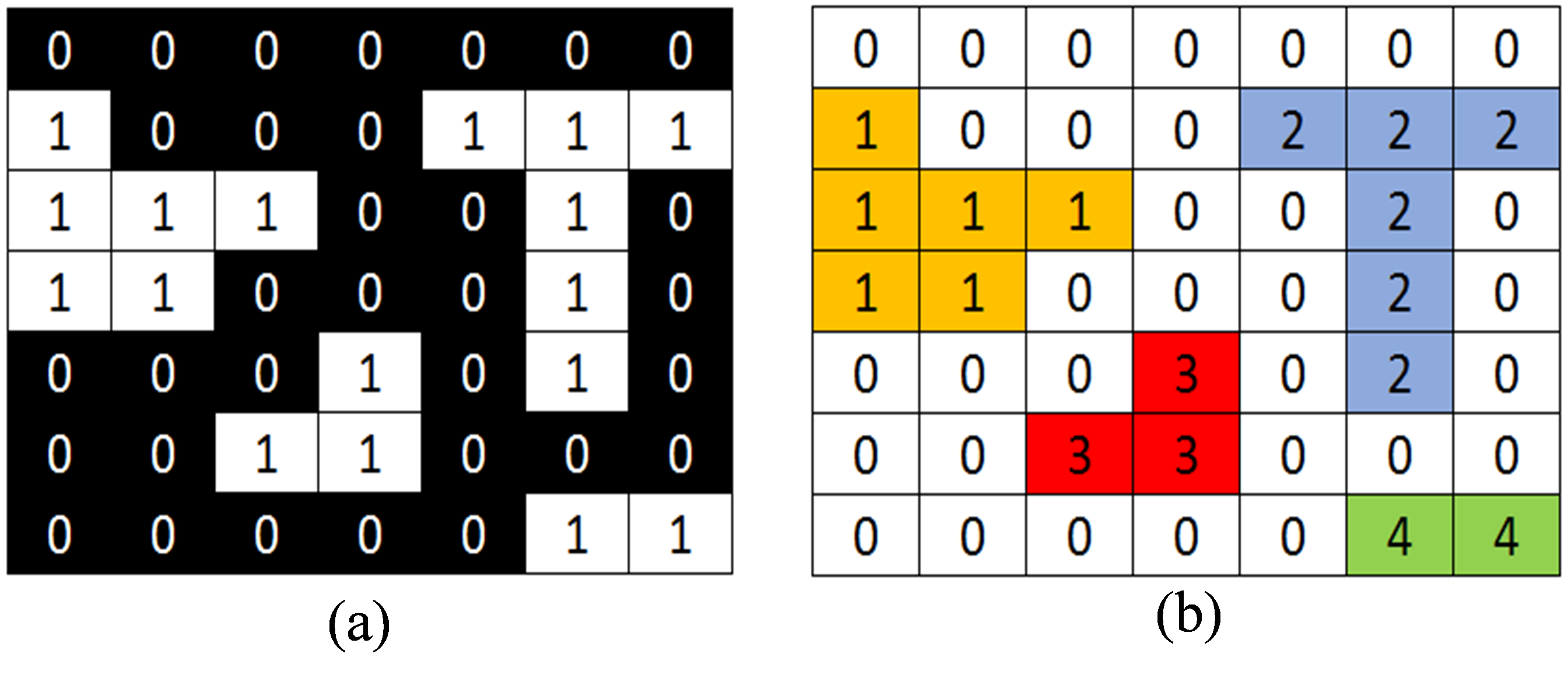
[labeled, numObjects] = bwlabel(BW);
[labeled, numObjects] = bwlabel(BW,n);
% n is the Connected search area, default: 8
Color-coding Objects : label2rgb()
Convert a label matrix into an RGB color image
Visualize the labeled regions
RGB_label = label2rgb(labeled);
imshow(RGB_label);
Object Properties : regionprops()
Provides a set of properties for each connected component
data = regionprops(labeled,'basic');
Interactive Selection : bwselect()
Select objects using the mouse
objI = bwselect(BW);
imshow(objI);
Differentiation and integration
Polynomial
$$ f(x)=a_{n} x^{n}+a_{n-1} x^{n-1}+\cdots+a_{1} x+a_{0}, $$
$$ differentiation: f^{\prime}(x)=a_{n} n x^{n-1}+a_{n-1}(n-1) x^{n-2}+\cdots+a_{1} $$
$$ integration: \int f(x)=\frac{1}{n+1} a_{n} x^{n+1}+\frac{1}{n} a_{n-1} x^{n}+\cdots+a_{0} x+k $$
% enter a polynomial to Matlab
p = [an, an-1, .... ,a0];
polyval()
return the value of polynomial in the x
p = [1,2,3,4]; x = -2:0.01:5;
f = polyval(p, x);
plot(x,f);
polyder()
return the polynomial differentiation
p = [1,2,3,4];
polyder(p);
polyint()
return the polynomial integration
polyint(p, k);
Numerical
$$ Differentiation: f^{\prime}\left(x_{0}\right)=\lim _{h \rightarrow 0} \frac{f(x0+h)-f(x0)}{h} $$
$$ integration: s=\int_{a}^{b} f(x) d(x) \approx \sum_{i=0}^{n} f\left(x_{i}\right) \int_{a}^{b} L_{i}(x) d x $$
diff()
calculates the differences between adjacent elements of a vector
x = [1 2 5 2 1];
diff(x);
% return 1 3 -3 -1
% Numerical differentiation using diff()
% at a point
x0 = pi/2; h = 0.1;
x = [x0,x0+h];
y = [sin(x0), sin(x0+h)];
m = diff(y)./diff(x);

% within a range
h = 0.1;
x = [0:h:2*pi];
integral()
caculate the numerical integration
y = @(x) 1./(x.^3 - 2*x);
integral(y,0,2);
% caculate the integration from 0 to 2

% Double integral
integral2(f,begin1,end1,begin2,end2);
% two param: x from begin1 to end1 ; y from begin2 to end2

% Triple integral
integral3(f,begin1,end1,begin2,end2,begin3,end3);
integration
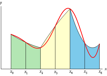
-
Midpoint rule
 $$
\int_{x_{0}}^{x_{3}} f(x) d x \approx h f_{0}+h f_{1}+h f_{2}=h \sum_{i=0}^{n-1} f_{i}
$$
$$
\int_{x_{0}}^{x_{3}} f(x) d x \approx h f_{0}+h f_{1}+h f_{2}=h \sum_{i=0}^{n-1} f_{i}
$$
$$ f_{0} = f\left(\frac{x_{0}+x_{1}}{2}\right) $$
Midpoint Rule Using sum()
h = 0.05; x = 0:h:2;
midpoint = (x(1:end-1) + x(2:end))./2;
y = f(midpoint);
s = sum(h*y);
-
Trapezoid Rule
 $$
\int_{x_{0}}^{x_{3}} f(x) d x \approx h \frac{f_{0}+f_{1}}{2}+h \frac{f_{1}+f_{2}}{2}+h \frac{f_{2}+f_{3}}{2}
$$
$$
\int_{x_{0}}^{x_{3}} f(x) d x \approx h \frac{f_{0}+f_{1}}{2}+h \frac{f_{1}+f_{2}}{2}+h \frac{f_{2}+f_{3}}{2}
$$
$$ f_{0}=\frac{f\left(x_{0}\right)+f\left(x_{1}\right)}{2} $$
Trapezoid Rule Using trapz()
h = 0.05; x = 0:h:2;
y = f(x);
s = h*trapz(y);
-
Second-order Rule : 1/3 Simpson’s
 $$
\int_{x_{0}}^{x_{2}} f(x) d x \approx \frac{h}{3}\left(f_{0}+{4 f_{1}}+{{f_{2}}}\right)
$$
$$
\int_{x_{0}}^{x_{2}} f(x) d x \approx \frac{h}{3}\left(f_{0}+{4 f_{1}}+{{f_{2}}}\right)
$$
Equation rooting
Symbolic Root Finding Approach
Using sym or syms to create symbolic variables
syms x
x = sym('x')
Function sovle finds roots for equation
syms x
y = x*sin(x)-x;
solve(y,x)
% return the ans of y = 0

% Solving Multiple Equations
syms x y
eq1 = x - 2*y + 5;
eq2 = x + y - 6;
A = solve(eq1,eq2,x,y);

% Solving Equations Expressed in Symbols
syms x a b
solve('a*x^2-b') % express x in terms of a and b
solve('a*x^2-b', 'b') % express b in terms of a and x
Symbolic Differentation and Integration
-
Symbolic Differentation : diff()
syms x y = 4*x^5; yprime = diff(y) % 20*x^4 -
Symbolic Integration : int()
syms x;
y = x^2*exp(x);
z = int(y);
z = z - subs(z, x, 0);
% subs is substitue 0 for x in z
Numeric root solver
fsolve()
f = @(x) (2*x + sin(x));
fsolve(f,0);
% f is a function handle
% 0 is initial guess
fzero()
it can’t solve tangent curve question
options
set params for fsolve or fzero
f = @(x) x.^2
options = optimset('MaxIter', 1e3, 'TolFun', 1e-10);
% MaxIter is number of iterations
% TolFun is Tolerance
fsolve(f,0.1,options);
fzero(f,0.1,options);
Finding Roots of Polynomials
Using roots()
roots only work for Polynomials
roots([1,2,3,4,5]);
Linear equation
$$ \left{\begin{array}{l} 3 x-2 y=5 \ x+4 y=11 \end{array}\right. $$
$$ \underbrace{\left[\begin{array}{cc} 3 & -2 \ 1 & 4 \end{array}\right]}{A}\underbrace{\left[\begin{array}{c} x \ y \end{array}\right]}{x} =\underbrace{\left[\begin{array}{c} 5 \ 11 \end{array}\right]}_{b} $$
Matrix Decomposition Factorization
- qr : Orthogonal-triangular decomposition
- ldl : Block LDL’factorization for Hermitian indefinite matrices
- ilu : Sparse incompelete LU factorization
- lu : LU matrix factorization
- chol : Cholesky factorization
- gsvd : Generalized singular value decomposition
- svd : Singular value decomposition
Matrix Left Division
Solving systems of linear equations Ax = b using factorization methods
Using / or mldivide()
A = [1 2 1;2 6 1;1 1 4];
b = [2; 7 ; 3];
x = A/b;
Cramer’s(Inverse) Method
$$ A A^{-1}=A^{-1} A=I $$
$$ x=A^{-1} b $$
Inverse Matrix
Using inv()
A = [1 2 1;2 6 1;1 1 4];
b = [2; 7 ; 3];
x = inv(A)*b;
Functions to Check Matrix Condition
Inverse matrix maybe not exist
Using cond() : Matrix Condition number
A = [1 2 3;2 4.0001 6;9 8 7];
cond(A);
Linear System
$$ \left{\begin{array}{l} 2 \cdot 2-12 \cdot 4=x \ 1 \cdot 2-5 \cdot 4=y \end{array}\right. \newline \newline $$
Eigenvalues and Eigenvectors
$$ \boldsymbol{A} \boldsymbol{v}{i}=\lambda{i} \boldsymbol{v}{i},\lambda{i} \in \Re $$
$$ \boldsymbol{b}=\sum \alpha_{i} \boldsymbol{v}{i}, \alpha{i} \in \Re $$
$$ \boldsymbol{A} \boldsymbol{b}=\sum \alpha_{i} \boldsymbol{A} \boldsymbol{v}{i}=\sum \alpha{i} \lambda_{i} \boldsymbol{v}_{i} $$
Using eig() to get v and λ
[v, d] = eig(A);
% A = v*d*inv(v)
Statistics
Central Tendency
- mean : Average or mean value of array
- median : Median value of array
- mode : Most frequent values in array
- prctile : Percentiles of a data set
Range
- max : Largest elements in array
- min : Smallest elements in array
Variance
$$ Variance : s=\frac{\sum\left(x_{i}-\bar{x}\right)^{2}}{n-1} $$
$$ Standard-deviation:S=\sqrt{\frac{\sum\left(x_{i}-\bar{x}\right)^{2}}{n-1}} $$
- sld : Standard deviation
- var : variance
Skewness
A measure of distribution skewness

Using skewness() to get skewness
y = skewness(X)
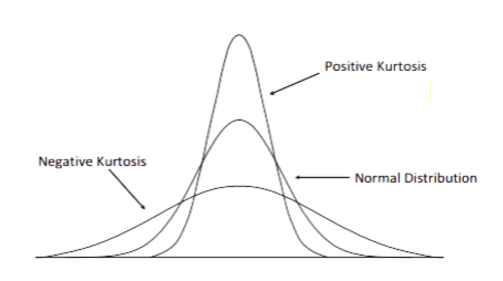
Kurtosis
A measure of distribution flatness
A Kurtosis of a normal distribution is zero
Hypothesis Test
Two-tailed Significance Test

One-tailed Significance Test

Common Hypothesis Test
- ranksum() : Wilcoxon rank sum test
- signrank() : Wilcoxon signed rank test
- ttest() : One-sample and paired-sample t-test
- ttest2() : Two-sample t-test
- ztest() : z-test
Polynomial Curve Fitting
Using polyfit()

x = [1 2 3 4 5];
y = [1 2 3 4 5];
fit = polyfit(x,y,1);
% return the confficients of f(x) = ax + b (order = 1)

% plot the f(x) and (x,y)
xfit = [x(1):0.1:x(end)]; yfit = fit(1)*xfit + fit(2);
plot(x,y,'bo',xfit,yfit);
Linearly Correlated
- scatter() : scatte plot
- corrcoef() : correlation , [-1,1]
x = [1 2 3 4 5];
y = [1 2 3 4 5];
scatter(x,y); box on; axis square;
corrcoef(x,y)
Multiple Linear Regression
Using regress()
X = [ones(length(x1),1) x1 x2];
b = regress(y,x);
% y = a + bx1 + cx2
Curve Fitting Toolbox
Using cftool() to open Toolbox
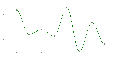
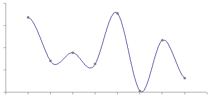
Interpolation
-
Linear
-
cosine
-
Cubic
-
Hermite
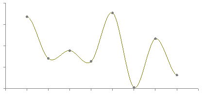
Common Interpolation approaches
- interp1() : 1-D data inerpolation
- pchip() : Piecewise Cubic Hermite Interpolation Polymial
- spline() : Cubic spline data interpolation
- mkpp() : Make piecewise polynomial
x_m = 0:0.5:2*pi;
y_m = cos(x);
x = 0:0.1:2*pi;
y = interp1(x_m,y_m,x);
plot(x_m,y_m,'.','color','g');
hold on;
plot(x,y,'.','color','r');
hold off;
(to be continued…)